Introduction

Previously we have written about the creation of infinite impulse response filter speaker cabinet models. This article covers a method for creating impulse response models which are more accurate and can be created for a variety of acoustic systems such as speakers and reverberant rooms.

“What’s an impulse reponse model?” You ask? In short it is a signal which allows very close recreation of a physical system’s acoustic properties. It is a high accuracy method by which, say, a guitar speaker cabinet can be modelled digitally. The impulse response data contains all of the tone response detail of the original device with, theoretically, no approximation.

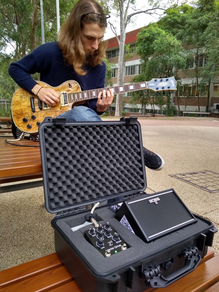
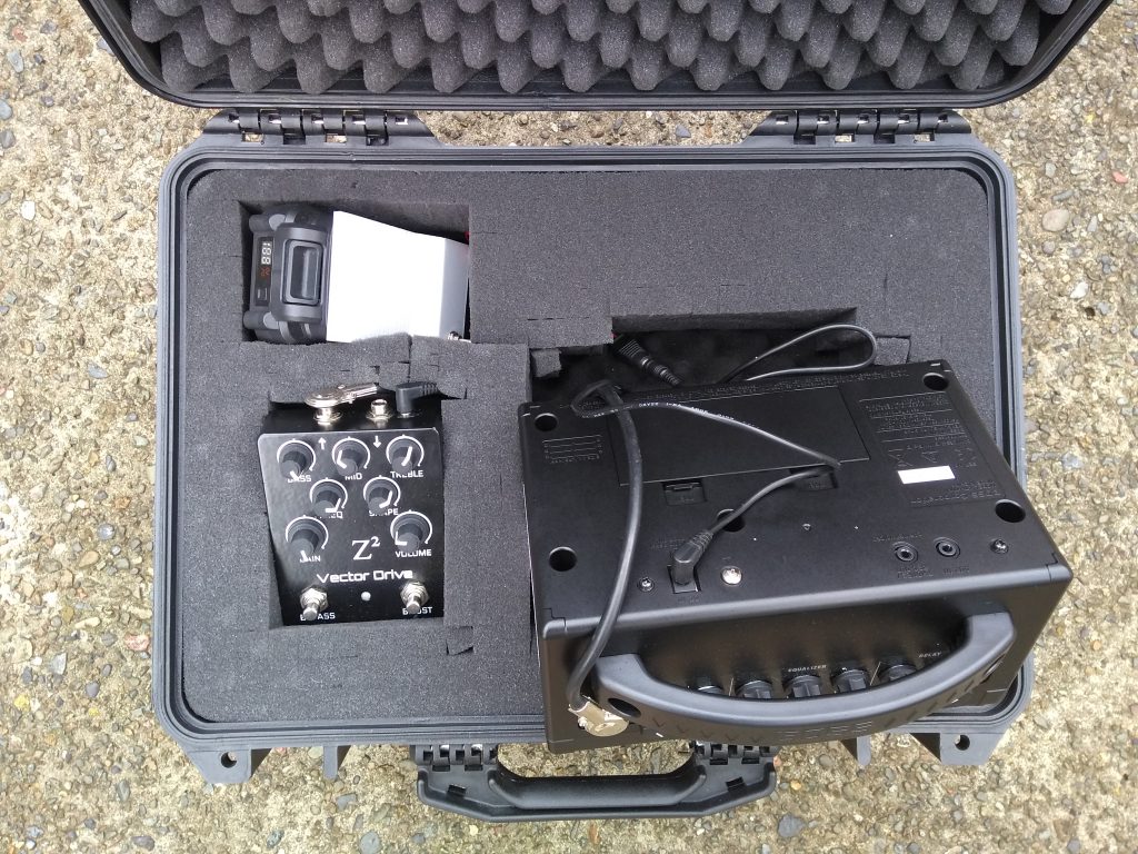
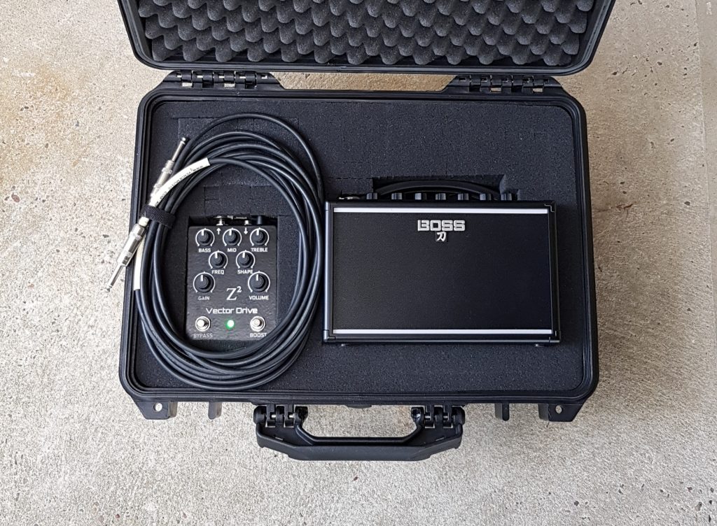
Lets start with the results. The audio clip below contains four copies of a short riff. One sample was created by recording the raw output of a Vector Drive distortion pedal and playing it back through a Fender Hotrod Deluxe III mic’ed up with a Sennheiser e906. The other three were created digitally using impulse response models of varying length.

Can you tell which is which? They aren’t identical but the differences are quite subtle. Which one is the real amp is obvious if you view a spectrogram of the file (spoiler: its the first one); there is high frequency (>15kHz) white noise present in the “real” recording which doesn’t exist in the modelled copies. There is also a small amplitude difference between each one as they were scaled to keep the peaks equal, not the RMS amplitude.

For reference, the clip below is a recording of the raw output from the Vector Drive. Really needs a cab after it, doesn’t it?

Great, how do we make an impulse response model?

The procedure is reasonably straight forward; all the complexity is buried in the underlying theory, discussed later. Following from the introduction the procedure here will demonstrate how to build an impulse response model for a guitar amplifier. NB: This procedure is provided for educational purposes only and is not guaranteed to be fit for purpose.

The minimum hardware requirements are:

A linear chirp generator (eg: Audacity and PC sound card)
Cables to connect the audio source to the amp/speaker cab
A microphone to record the speaker (NB: the microphone’s (and rooms!) response will be included in this model. It captures everything)
Octave (free)

Procedure:

Open Audacity and generate a linear chirp. Recommended settings are 10Hz to 22kHz, 1 second length, 0.8 to 0.8 amplitude (ie: constant, not fading). The sample in the introduction was created with a 1 second chirp and the code below assumes a 1 second chirp (48kHz sample rate).
Leaving some blank space, append a short (50-100ms) tone burst after the chirp. This will be used as a timing marker.
Connect the sound card to the amp’s input.
1. (Optional) This method will capture the amp’s EQ settings. You can set them up as you like or plug the signal source into the PA in / FX loop to bypass the preamp circuits.
Ensure that the amp is running on the clean channel. Distortion will result in a poor model.
Run a test recording to set the sound card’s output level. This is a balancing act between noise (if the drive is too low) or distortion (if it is too high).
Play the chirp and record the microphone simultaneously
Using the short tone burst align the tracks to compensate for any sound card latency. This also removes latency due to the speaker->mic air gap. Don’t worry about any trailing microphone noise/silence, it will be cut off in Octave.
Export the chirp track, call it input.wav
Export the recorded track, call it output.wav
Copy the .wav files to the same folder as the code below and open Octave

With the input and output data saved in .wav files we can build the impulse response in Octave. Assuming that a 1 second chirp sampled at 48kHz was used the following code will open the files, extract the recording of interest and plot the “full” impulse response:

x = audioread('input.wav')';
y = audioread('output.wav')';
t1x = x(1:48000); % Extract just the first second
t1y = y(1:48000); % of the chirp and recorded audio

IR = conv(fliplr(t1x), t1y, 'same'); % Perform the convolution to create the impulse response
plot(IR) % Plot it for inspection

If you’d like to repeat this with our test data it can be downloaded here: output.wav input.wav.

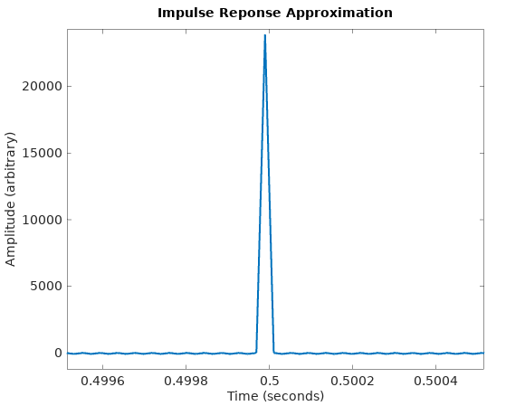
The script above then provides the following plot of the amp’s impulse response:

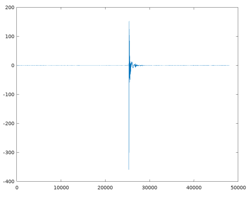
In its current form it will produce a high accuracy model of the amp but many of the 48000 samples present can be ignored without a significant error. The final sample in the introduction was created with this data truncated to only 1000 samples! Zooming into the graph we can obtain the array index for when the impulse starts, I’ll choose index 25330.

The “end” is a little harder to choose because there is a long, slowly decaying, tail. In reality this tail only significantly impacts subsonic frequencies so much of it can be truncated. Choosing by eye, lets go with sample 27000.

This block can then be extracted, normalised to +/-1, and saved:

IR = IR(25330:27000);
audiowrite("impulse.wav", IR/max(abs(IR)), 48000);

Using the impulse response

So we have an impulse, what now? Applying this IR model to a .wav file in Octave requires it to be convolved with a previously made recording (in our example: raw output from a guitar pedal):

input = audioread("recording.wav");
IR = audioread("impulse.wav");
result = conv(input, IR, 'same');
audiowrite("output.wav", result, 48000);

Alternatively, the impulse response can be loaded into a suitable VST plugin and used in your normal DAW workflow.

Theory: What actually is an “impulse response model”? (Math warning!)

In linear system theory any system (be it a circuit, speaker, acoustically interesting room, etc) can have its frequency response fully characterised by its so-called impulse response, $h(t)$ . This system’s output, $y(t)$ , due to an arbitrary input, $x(t)$ , can then be calculated via a convolution operation as follows:

$y(t) = x(t) * h(t) = \int_{-\infty}^{+\infty} x(\tau)h(t-\tau) d\tau.$

It turns out that $h(t)$ is an incredibly useful signal to obtain. It contains all the linear frequency response characteristics of a particular system without any approximation. Theoretically, an impulse response model is the most accurate linear (ie: non-distortion) model possible.

Mathematically, the impulse response is the signal generated by the system when the input is an infinitely high, instant, pulse known as a dirac delta function, $\delta (t)$ .

“Uhhh, ok”, you say, “but how is that useful? Infinite pulses don’t exist!”. Good question! In reality we can’t drive a large bang through a guitar amp or speaker to model it for a variety of reasons (although popping balloons or starter pistols are used when analysing room reverb) however, it turns out that $\delta(t)$ has a very useful property which we can emulate in other ways; its Fourier transform is simply:

$\delta(t) \xrightarrow{\mathcal{F}} 1.$

The practical interpretation of this is that $h(t)$ is the output of the system when every frequency is thrown into the system simultaneously. Engineers, being practical people, approximate this by creating other test signals which contain the full frequency spectrum of interest spread out in time. In a “hand-wavy” way practical test signals are dirac deltas which have been dispersed. The phase of each frequency has been shifted to spread out the signal’s energy across a finite, non-zero, amount of time.

Test Signal Creation & Analysis (Further Maths Warning!)

Lets explore one of the simpler test signals: a linear chirp. This is a sine function with a frequency which varies from $f_0$ to $f_1$ over a time period $T$ in a linear fashion. Assuming an initial phase of zero, it can be directly calculated as a function of time, $t$ , as follows:

$\sin \left[ 2 \pi \left( f_0 t + \frac{k}{2} t^2 \right) \right]$

where

$k = \frac{f_1 - f_0}{T}.$

We will use the above formula for analysing the signal’s properties in Octave but in practice you’d probably just use Audacity’s built-in chirp creation function.

To explore the frequency domain properties of the linear chirp run code below. It creates a 1 second long linear chirp from 2kHz to 20kHz. A real test signal would start at a lower frequency (say, 20Hz) but this one is limited for demonstration purposes.

T = 1; % Length, seconds
Fs = 48e3; % Samplerate
t = linspace(0,T, T*Fs);

f0 = 2000;
f1 = 20e3;
k = (f1-f0)/T;

phi = 2*pi*(f0*t + k/2*t.^2);
x = sin(phi);

With the signal created a bunch more code is used to make nice looking plots of its Fourier transform’s amplitude and phase:

set(0, 'defaultaxesfontsize', 14)
figure(1)
hold off
subplot(2,1,1)
plot(f,fftshift(abs(fft(x))), 'linewidth', 2);
axis([min(f) max(f)]);
xlabel('Frequency (Hz)', 'fontsize', 14);
ylabel('Amplitude (arbitrary)', 'fontsize', 14);
title('Chirp Amplitude Vs Frequency', 'fontsize', 14);
subplot(2,1,2)
hold off
plot(f,fftshift(unwrap(arg(fft(x)))), 'linewidth', 2);
axis([min(f) max(f)]);
xlabel('Frequency (Hz)', 'fontsize', 14);
ylabel('Phase (radians)', 'fontsize', 14);
title('Chirp Phase Vs Frequency', 'fontsize', 14);

and we get the resultant plot:

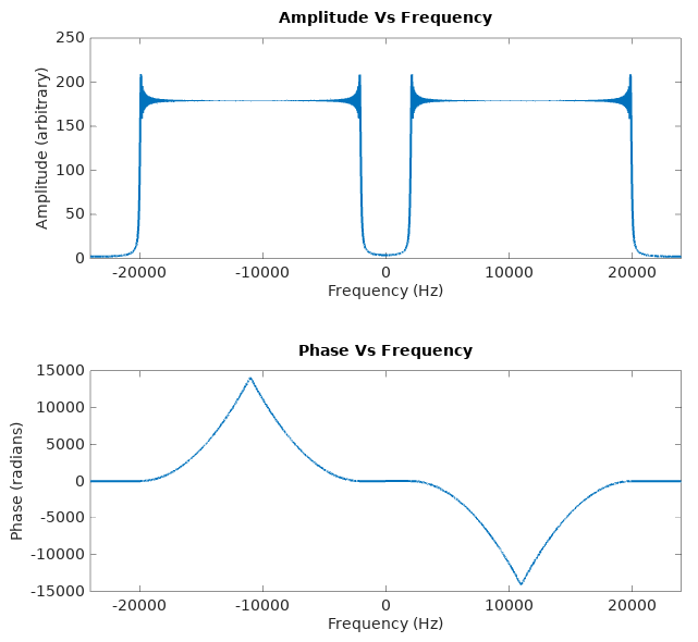
Remember how the Fourier transform of $\delta (t)$ was just $1$ ? That would be a constant horizontal line on the amplitude and frequency plots. Here we have, within a given frequency range, an amplitude plot which is a good approximation of a horizontal line. There is some strong Gibbs phenomenon around the corners but this error becomes less significant if the chirp is longer (eg: 60 seconds). The start and stop frequencies of the chirp are also arbitrary; we can choose them to be outside of the frequency range of interest so the error becomes insignificant for the device we are measuring.

The phase, however, is obviously not a straight line because the signal’s frequency content is spread out over 1 second instead of all being delivered instantaneously.

So how does this help us get an impulse response? To get from here to an impulse we need to perform some kind of manipulation which removes the frequency dispersion. The result of this would be a phase plot which is a straight line (not necessarily a horizontal one, however, as a pure time delay on $\delta(t)$ results in a linear phase response. ie: a straight line with some non-zero gradient).

Due to the phase plot’s anti-symmetric nature (ie: it is an odd function) it can be flattened by multiplying the chirp’s Fourier transform by the frequency reversed copy of itself. This can also be achieved with a time domain reversal, due to the Fourier transform property:

$x(-t) \leftrightarrow X(-\omega).$

That multiplication would be straight forward, and relatively computationally efficient, but it is worth noting the Fourier transform property which states that a frequency domain multiplication is equivalent to a time domain convolution:

$x(t) * y(t) \leftrightarrow X(\omega)Y(\omega)$

. This just allows the impulse response creation algorithm above to be purely in the time domain, simplifying the code.

So lets try it; taking our 2kHz to 20kHz linear chirp from before and convolving it with the time-reversed copy of itself can be done with:

conv(x, fliplr(x), 'same');

Plotting the result, and zooming in, produces:

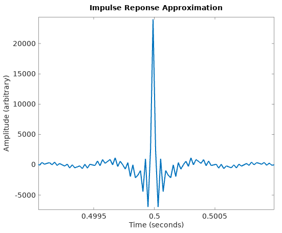Far from an ideal impulse but it certainly has the “big spike over a short time” property. This is, to a first approximation, a delta function which has been band-pass filtered (ie: it is the impulse response of a band-pass filter). Within the 2-20kHz frequency range it is a good approximation of a delta and outside that range it is essentially useless.

Repeating all the above analysis with a 0Hz to 24kHz chirp (ie: one which covers the full frequency range possible when sampling at 48kHz) results in:

which is getting far closer to an ideal delta function.

There is one final ingredient needed before we can model real systems: it will be assumed (and proven later) that passing the linear chirp through the system of interest then performing the above time-reversal and convolution results in a good approximation of the system’s impulse response.

Deconvolution Via Inverse Elements

The previous section defined the linear chirp signal, $x(t)$ and developed another signal, $x^\prime (t)$ which had the property:

$x(t) * x^\prime (t) \approx \delta(t).$

Mathematically speaking, $x^\prime (t)$ is the inverse element of $x(t)$ under a convolution operation.

Following is a proof that if such a signal, $x^\prime (t)$ exists then $x(t)$ becomes an excellent candidate for measuring a system’s impulse response, $h(t)$ .

Given that the output, $y(t)$ of a system with (unknown) impulse response $h(t)$ due to input $x(t)$ is:

$y(t) = x(t) * h(t)$

we can use $x^\prime (t)$ to identify $h(t)$ via a further convolution operation:

$h(t) \approx y(t) * x^\prime (t).$

Proof:

$\begin{align*} h(t) &\approx y(t) * x^\prime (t) \\ &= x(t) * h(t) * x^\prime \\ &= (x(t) * x^\prime (t)) * h(t) ~&\textrm{Associativity} \\ &\approx \delta(t) * h(t) \\ &= h(t)~&\textrm{Multiplicative identity}.\end{align}$

Proofs of the convolution operator’s associativity and multiplicative identity properties can be found on Wikipedia.

Creation of $x^\prime (t)$ must be manually done for each particular test signal. For the linear chirp it has been shown above that time reversal via left-right flipping of $x(t)$ creates $x^\prime (t)$ (NB: the linear chirp’s equation is non-linear in time so $t$ can’t simply be substituted as $-t$ ).

A final note: in all the analysis here the amplitudes of the various signals has been ignored. You may have observed that all amplitude plots scales have been arbitrary, scaling of the resultant signals has been done manually to avoid saturation and overflow in the audio files.

Other Deconvolution Methods

So far all the discussion has assumed that it was practical to inject an arbitrary test signal into the system, but what if this isn’t possible? What if we only had, say, input/output recordings of guitar playing and couldn’t access the equipment they were made from?

The procedure in this circumstance is to use some kind of deconvolution process. A naive deconvolution observes that if

$y(t) = x(t)*h(t) \leftrightarrow Y(\omega) = X(\omega)H(\omega)$

then $H(\omega)$ can be found as

$H(\omega) = \frac{Y(\omega)}{X(\omega)}$

and $h(t)$ calculated as the inverse Fourier transform of $H(\omega)$ .

The downfall of the above approach is that noise becomes a major problem. At frequencies where $X(\omega)$ is “very small” the value of $H(\omega)$ will be “very large” and dominated by noise in the measurement of $X(\omega)$ .

One solution to the noise problem is the Wiener deconvolution. This method, in a hand-wavy way, intentionally attenuates $H(\omega)$ for frequencies with poor signal to noise ratio. The Wiener deconvolution minimises mean square frequency domain error under the assumption that the noise is distributed as a Gaussian with mean zero.

The solution to noise presented in this article was to ensure that the frequency spectrum $X(\omega)$ had sufficiently high SNR at all frequencies of interest. Furthermore, the use of the deconvolution function (time reversed linear chirp) removes the need to perform a division, further attenuating noise.

Other Test Signals

Linear chirps are not the only (nor even the best) test signal for impulse response creation. An exponential chirp, for example, has the advantageous property that it separates the impulse response of each distortion harmonic. Mildly non-linear systems (such as power amps) can then have their distortion characteristic removed from the measurement. Distortion measured with a linear chirp tends to manifest itself as noise and can’t be separated. The compromise is that an exponential chirp requires more manipulation, which the following Octave code demonstrates without proof:

len = 1; % Chirp length
Fs = 48e3; % Sample rate
f0 = 20; % Lower frequency
f1 = 12000; % Upper frequency
t = linspace(0,len,Fs*len); % Time vector

% log sweep creation
k = (f1/f0)^(1/len);
x = sin(2*pi*f0*( (k.^t - 1) / log(k)));

% Build deconvolution function (inverse element of "x")
k2 = -6*log2(f1/f0);
env = -k2/len*t + k2;
env = 10.^(env/20);
d = fliplr(x.*env);

% Pass signal "x" through the system to be measured
% Call measurement "y"
% IR = conv(y, d); then creates impulse response

At this time the details of impulse response creation with log sweeps is lefts as an exercise for the reader.

There have also been efforts to use maximum length sequences for audio system identification. This is a type of pseudo-random noise generator where a system’s impulse response can be calculated with a time domain cross-correlation (a very close relative of convolution).

Author: Z² DSP

Speaker Cab Modelling Part II: Impulse Response Modelling, Theory and Practice

Introduction

Great, how do we make an impulse response model?

Using the impulse response

Theory: What actually is an “impulse response model”? (Math warning!)

Test Signal Creation & Analysis (Further Maths Warning!)

Deconvolution Via Inverse Elements

Other Deconvolution Methods

Other Test Signals

Further Reading

Portable Demo Setup

Vector Drive: Quick Start Guide

Drive Mode

Advanced Tuning

Drive Tuning

‘Input High Pass Filter’

‘Input Low Pass Filter’

Clean Mix

Mix

Clean EQ

Internal Memory