Overdrive: What is it and how is it implemented in the Vector Drive? Part One

Introduction

Overdrive is at the heart of modern guitar playing. We all know what it sounds like; from the hint of breakup as tubes begin saturating, to the mighty crunch and roar of an amp being pushed by a boost pedal. Whether you play blues, rock, psych, metal or industrial-post-noise-core, you’ll need an overdrive which can give you what you’re looking for.

Understanding the causes and characteristics of overdrive in amplifier electronics is crucial to making a quality pedal that delivers versatile overdrive. In this article, we show you some of our research and inspiration for development of our algorithms.

The first section will show analysis of a classic solid state overdrive circuit and how the Vector Drive distortion pedal models this effect. The second half of the post will look at measurements from a tube amplifier pushed into saturation along with the Vector Drive’s wave shaping feature which can mimic this.

Classic Overdrive Pedal Analysis

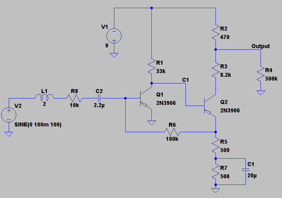
Lets begin this section by looking at the core of traditional overdrive pedal circuits. Below is a typical overdrive clipping circuit, such as that in the Tube Screamer, built in LTSpice. The circuit has been simplified by removing all frequency dependent components and using ideal diodes and op-amp. As with our fuzz analysis we’re stripping everything back to its core to understand the essence of an effect, not copy an existing product.

NB: Non-ideal (ie: real) diodes produce a much smoother clipping than is presented here but ideal diodes make the circuit’s underlying behaviour easier to see.

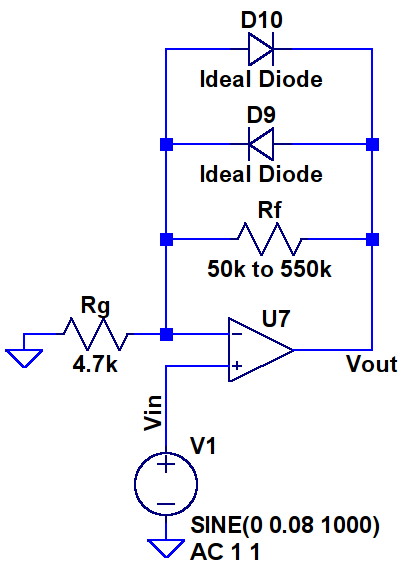The circuit above is based around an op-amp in a so-called non-inverting topology which, without the diodes, has a gain of:

(1) $\begin{equation*}Gain=1 + \frac{R_f}{R_g}.\end{equation*}$

The resistor $R_f$ is what is adjusted when turning the gain knob on an overdrive pedal.

If the diodes are ignored and the typical 50k to 550k resistance range is used the circuit above has a gain of between 9.5 and 118, or approximately 20dB to 41dB. With this much gain a typical 300mV guitar signal would be amplified to between 3V and 30V, enough for the op-amp’s output to hard clip near its power supply voltage (typically 0-9V). We will see later that situation is avoided by the diodes.

For the following analysis we will assume the diodes are ideal, this means that if their forward voltage is below some threshold, we chose 0.6V, their resistance is infinite and if it is above 0.6V their resistance becomes zero.

The diodes avoid hard clipping by reducing the circuit’s gain when the output reaches a certain amplitude. The gain reduction occurs because when one of them conducts the effective value of $R_f$ drops to zero, causing unity gain as per the equation above.

Given that the diodes conduct when their voltage exceeds 0.6V we need a way of finding their terminal voltage as a function of $V_{in}$ . The voltage across the diodes can by calculated by noting the characteristics of ideal op-amps and concluding that the inverting (-) and non-inverting (+) inputs of the op-amp will always be the same voltage. Therefore we claim that the op-amp’s inputs will both be equal to $V_{in}$ (the input voltage) and, considering the case where $V_{in} > 0$ the diode D9 will conduct when:

(2) $\begin{align*} V_{out} -V_{in} &\geq 0.6 \\ V_{out} &\geq 0.6 + V_{in}.\end{align*}$

The same logic can be used to derive the equation for D10’s conduction threshold as $V_{out} \leq 0.6 - V_{in}$ but the proof is left as an exercise for the reader.

Given equation 2 and the fact that a conducting diode drops $R_f$ to zero (and the gain to 1) we can conclude that if D9 is conducting then $V_{out}$ is, in fact, equal to $0.6 + V_{in}$ . ie: the output is clamped by the diode’s conduction threshold.

The diode’s conduction requirement can be written in terms of $V_{in}$ by observing that:

(3) $\begin{align*}Gain &= \frac{V_{out}}{V_{in}} = 1 + \frac{R_f}{R_g} \\ &\Rightarrow V_{out} = V_{in}\left(1 + \frac{R_f}{R_g}\right)\end{align*}$

and substituting this expression for $V_{out}$ into equation 2:

(4) $\begin{align*} V_{out} &\geq 0.6 + V_{in} \\ V_{in}\left(1 + \frac{R_f}{R_g}\right) &\geq 0.6 + V_{in} \\ V_{in}\left(1 + \frac{R_f}{R_g}\right) - V_{in} &\geq 0.6 \\ V_{in} \frac{R_f}{R_g} &\geq 0.6 \\ V_{in} &\geq 0.6 \frac{R_g}{R_f} \end{align*}$

We can now write a complete set of equations for the overdrive circuit:

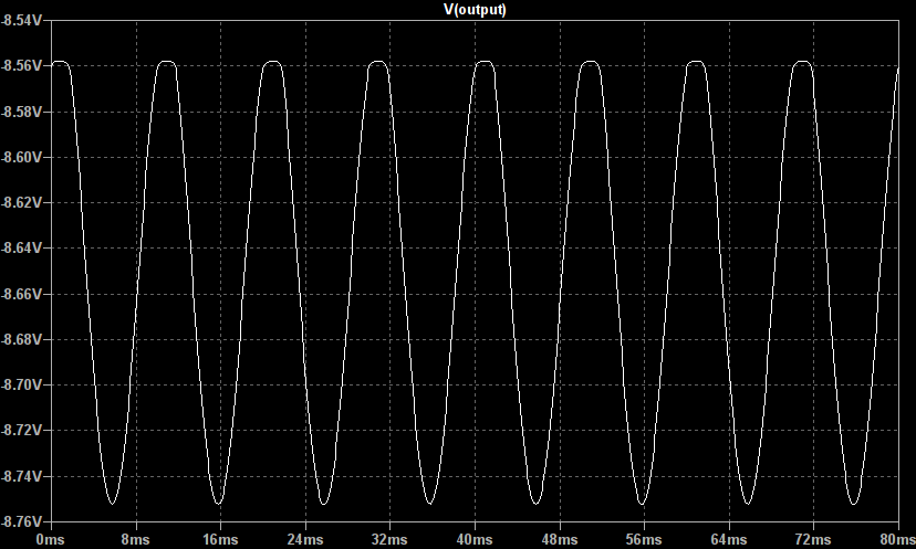
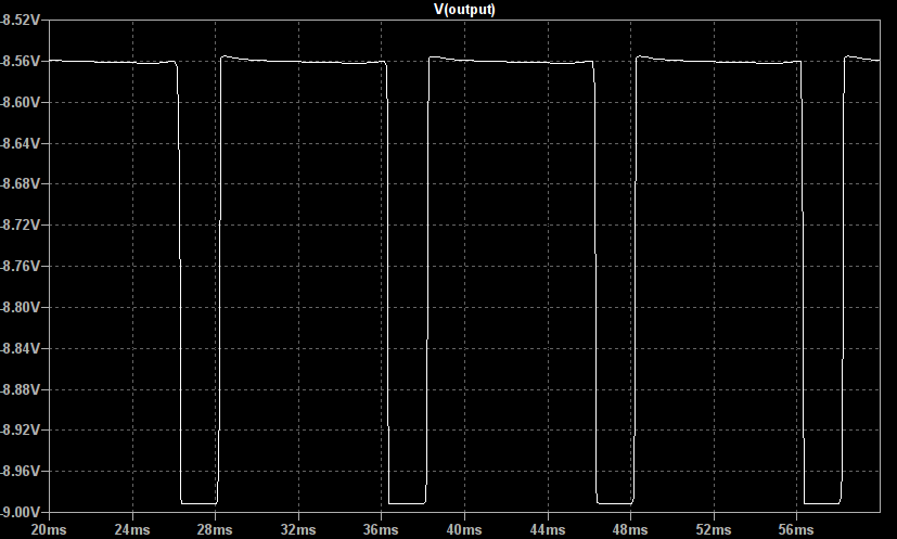
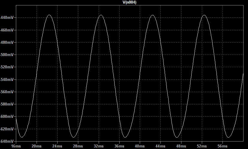
(5) $\begin{equation*} V_{out} = \begin{cases} \left( 1 + \frac{R_f}{R_g} \right)V_{in} &, V_{in} < 0.6 \frac{R_g}{R_f} \\ 0.6 + V_{in} &,V_{in} \geq 0.6 \frac{R_g}{R_f} \end{cases} \end{equation*}$

So, if the input is driven with a sine wave the general shape of the output is shown below:

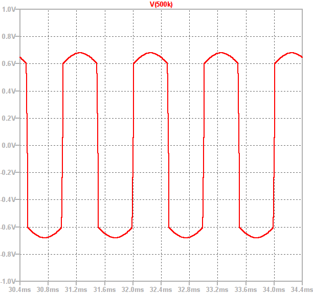
It can be seen that between approximately -0.6V and 0.6V the output is a sine wave which has been amplified with high gain. However, as soon as the output exceeds $0.6+V_{in}$ the diodes conduct and the gain drops to 1. This causes the output to follow the input, shifted by +/- 0.6V. This creates smooth peaks instead of a hard clipped square wave.

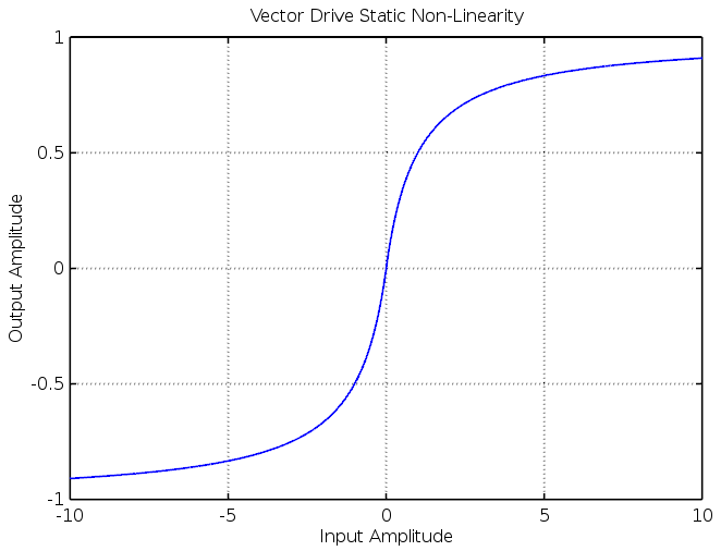
Another way of visualising the circuit’s behaviour is by plotting the input signal’s amplitude on the x-axis and the corresponding output amplitude on the y-axis to create a graph of the circuit’s static non-linearity. The plot below shows this for three different values of $R_f$ :

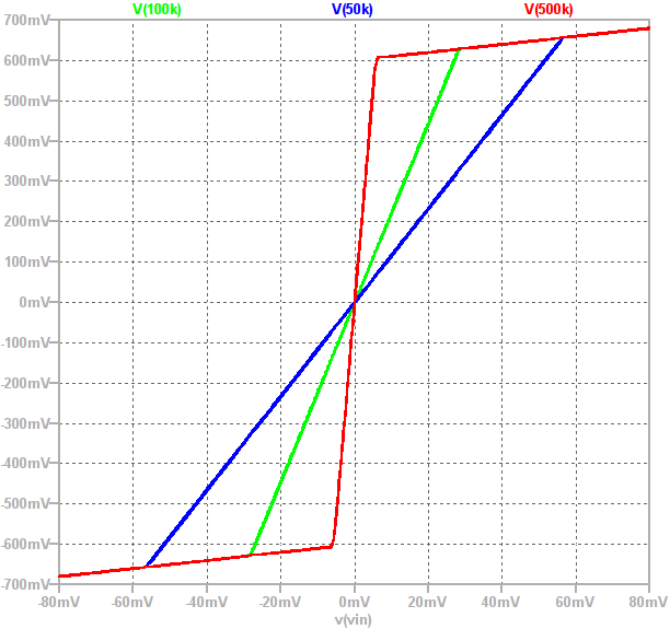
Observe that the “knee point” is at $(V_{in}+0.6)~V$ . The gain of a circuit is equal to the gradient of the above plot and the two gain “regions” can clearly be seen. The gain is high when the output is between $\left(0.6 + V_{in}\right)~V$ and $(-0.6 + V_{in})~V$ then suddenly drops to 1 once one of the diodes conducts.

The broad effect of this circuit is a type of smooth clipping where the “smoothness” comes from the clean input being mixed in with the distorted output. This is, in fact, the core feature of overdrive: it is a saturated signal with some clean input mixed back in.

This can be seen from the circuit’s gain equation:

(6) $\begin{align*}Gain &= \frac{V_{out}}{V_{in}} = 1 + \frac{R_f}{R_g} \\ V_{out} &= V_{in} \times \left(1 + \frac{R_f}{R_g}\right) \\ &= V_{in} + V_{in} \times \frac{R_f}{R_g}\end{align*}$

One way of looking at the circuit’s two operating regions is to imagine the value of $R_f$ varying with the input voltage. This equation then informally shows that the output, $V_{out}$ is equal to the clean input, $V_{in}$ plus a high gain copy of it where the high gain signal gets saturated (clipped) at the diode’s forward voltage. This supports the statement above that the overdrive effect is a saturated version of the input with some of the clean input mixed over the top.

The Vector Drive’s Overdrive Implementation

The basic signal chain of the Vector Drive’s overdrive effect is shown below:

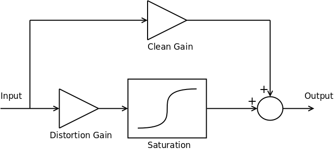
The full signal chain contains several filter blocks (such as the main 3 channel parametric tone controls) but these have been omitted for clarity.

In traditional overdrive pedals the distortion gain level, set by $R_f$ , is adjustable. In the Vector Drive, however, the versatility of DSP allows for both the distortion gain and clean gain to be set by the player.

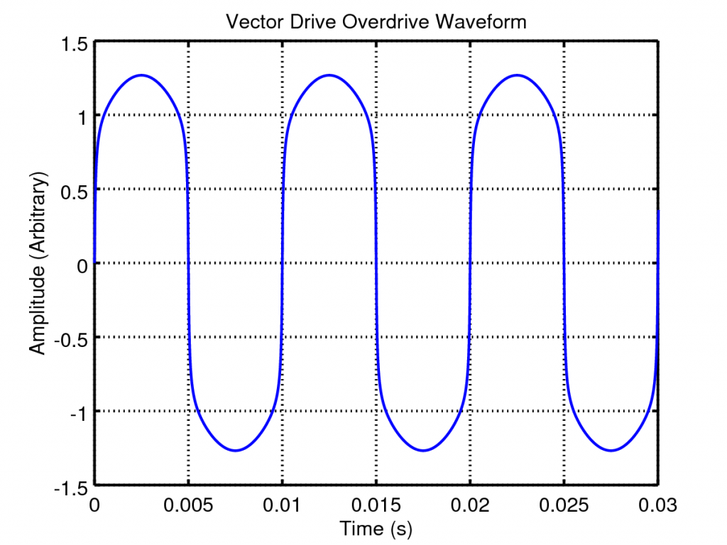
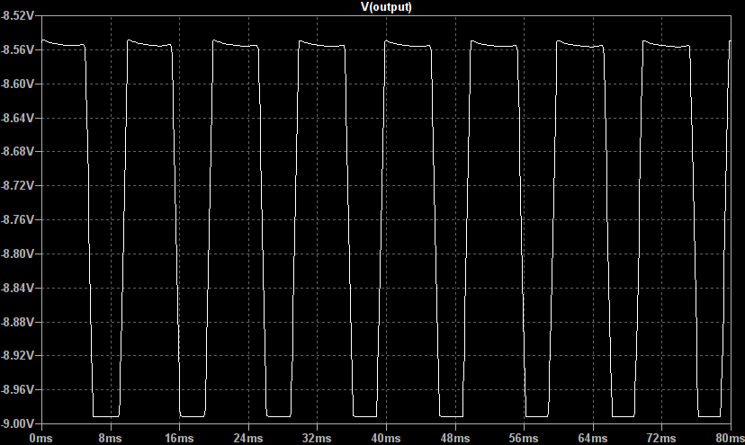
In our DSP code the saturation function is the smooth clipping equation:

(7) $\begin{equation*}y = \cfrac{x}{1 + \left| x \right|}\end{equation*}$

which, when mixed with the clean signal, results in waveforms such as the one below; a beautifully smooth clipped sine wave:

So lets look at the effect of varying the distortion and clean gains. If we plot the above waveform shaping as a static non-linearity and vary the distortion gain we get the following plots:

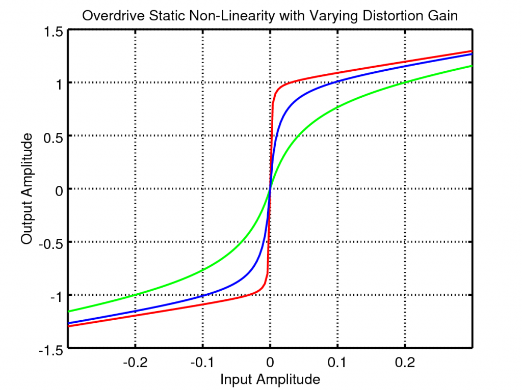The distortion gain adjusts the underlying tonal mix of the output, increasing this gain creates higher frequency harmonics leading to a more crunchy sound.

If, instead, we vary the clean mix the static non-linearity changes as follows:

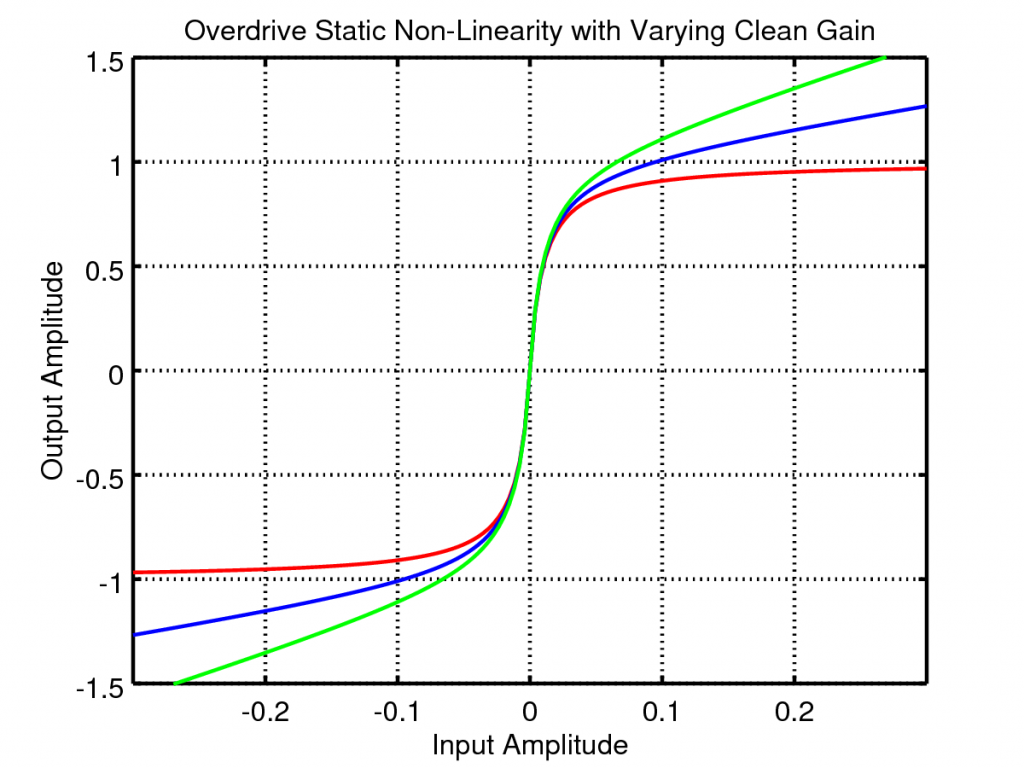
With this adjustment the output can be varied from totally saturated hard core distortion to super subtle overdrive.

September 4, 2017September 20, 2017

Modelling Fuzz

Introduction

Classic fuzz circuits, such as the one found in the original Fuzz Face pedal, created a unique style of asymmetric clipping which gave them their signature fuzzy feel. In this post we’ll be looking at the circuit feature which caused their hard clipped output waveforms to be asymmetric and how the Vector Drive can be used to recreate classic fuzz tones. We also demonstrate some sample audio and show how these features really sound.

We’d like to give a shout out to the excellent analysis of the Fuzz Face done by Electro Smash. Their articles were invaluable while designing the Vector Drive.

Fuzz Face Analysis

For this section we built the Fuzz Face circuit in LTSpice, a free (no cost, closed source) circuit simulation package from Linear Technology. The original Fuzz Face used the AC128 germanium PNP transistor, a device which doesn’t have a manufacture-published SPICE model (unless you trust random forum posts). As such we substituted The AC128 with a modern 2N3906 silicon PNP transistor. The results won’t exactly match the real circuit (the AC128s were highly variable anyway) but we aren’t trying to copy the Fuzz Face, just observe its general clipping style.

You can find our LTSpice circuit here. Note that it includes a 2H inductor and 10k Ohm resistor modelling the source impedance of a guitar pickup. These are typical values, if you can find data on your own pickup they can be adjusted to your needs. Note that active pickups, such as the classic EMG81, will have a purely resistive output impedance requiring the removal of L1.

The characteristic we’re interested in here is the shape of the output waveform at low and high input levels. Driven with a 1mV sine wave the output below shows a little clipping and is amplified to around 200mV p-p:

However, when driven with a larger 100mV signal the output shows obvious hard clipping and is strongly asymmetric, spending much of its time clipped high with only short bursts clipped low:

NB: The above plot was made with the pickup source impedance removed.

The source of this asymmetry is the way the input signal is coupled into the base of Q1, the first transistor. When driven with a 100mV sine wave the voltage at this point is only below the ~600mV base conduction threshold for a small amount of time at the bottom of each cycle:

It is crucial to note that here we are driving the Fuzz Face’s input with a low impedance source such as another guitar pedal. With the typical pickup model (10k resistor and 2H inductor) placed in series with the signal source the output becomes markedly more symmetric but still spends more time clipped high than low:

It is control over this hard clipped asymmetry (the non-50%-duty cycle) which we implemented in the Vector drive.

Vector Drive Implementation

Before talking about the asymmetry implementation we will look at the Vector Drive’s distortion signal chain. The input signal is fed through a high pass filter to remove any DC offsets (and, if desired, bass frequencies) then into a static non-linearity. The static non-linearity is the equation which dictates the signal clipping shape.

In the Vector Drive the static non-linearity is the equation:

(1) $\begin{equation*}y = \frac{x}{1 + \left| x \right|}\end{equation*}$

which, when plotted, looks like this:

This saturation function is reasonably soft but perfectly capable of producing hard clipped, high gain waveforms as well.

The Fuzz Face’s asymmetry can be produced by adding a vertical offset to the input signal prior to feeding it through the static non-linearity function. There are, however, complications. The result of adding a constant offset of 8 to input sine waves of amplitudes 1 (blue), 10 (green) and 100 (red) is shown below:

The green waveform is as expected, it shows strongly asymmetric soft clipping. However, the effect is lost on the high amplitude sine wave and the low amplitude input has been strongly attenuated. This offsetting method sounds markedly unpleasant as strong signals suddenly jump out and the ability to sustain notes is lost, as audible in the following sound clips:

NB: All the sound clips below have been passed through the Vector Drive’s cabinet modelling filter. No external amplifier has been used. The Vector Drive’s input high pass filter cutoff was set to 100Hz.

Clean recording:

Constant offset clipping:

The solution to the problem above is to measure the input’s amplitude with an envelope follower and add an offset which is proportional to this value. Adding an 80% amplitude offset to the three sine waves above produces this result:

The asymmetry is very similar between the three waveforms and the low amplitude input is only about 6dB below the hard clipped high gain waveform (ie: this method compresses dynamic range in a way we expect a distortion circuit should). The DC offset present in the above waveforms is easily removed with a low frequency (~20Hz) high pass filter.

When this method is applied to the sample riff above it produces a far more musical result. The following samples start with zero offset (just plain distortion saturation) and become “fuzzier” in each clip thereafter:

The Vector Drive allows the offset to be smoothly varied from purely symmetric distortion to super crackly “ripped speaker cone” fuzz. This parameter can be adjusted independently of the other major settings such as the input high pass filter, amplitude symmetry waveshaper and 3ch EQ allow full control of your custom tone creation.

September 1, 2017January 31, 2019

Speaker Cabinet Modelling Part I

This post covers the creation of infinite impulse response filters which emulate guitar speaker cabinets. A follow-up post covers the creation of more accurate, but far more computationally intensive, impulse response models.

Introduction

On the Vector Drive’s long list of features is cabinet emulation; the ability of the pedal to generate an output which sounds like it is coming from a real amp’s speaker cabinet. This is done by passing the output audio through a series of filters which mimic the tonal properties of a guitar speaker we have in the Z Squared DSP studio: a Blackheart BH112 1×12″ driven by a Little Giant 5 tube head.

This post describes the method we used to tune the cabinet emulation system, a series of four second order infinite impulse response (IIR) filters. These are digital signal processing (DSP) filters which models analog RLC circuits and are used here because of their computational efficiency and low latency. If you’ve used digital audio workstation cab emulation plugins they may instead use finite impulse response (FIR) filters or even convolutions. These methods can be more accurate but typically introduce unacceptably high delays (ie: they aren’t real-time methods) and are far too computationally intensive for the humble DSP microcontroller in the Vector Drive.

The goal of our cabinet modelling procedure was therefore to create a high order IIR filter which closely approximated the sinusoidal steady state response of the BH112 speaker cabinet. This model ignores any non-linear (distortion) effects of the speaker/amp combo (ie: measurements are performed at a low-ish volume) and only applies to a single microphone location.

Audio Samples

Before diving into the details have some audio samples, this is probably what most readers are here for anyway. The following clips compare the same audio with & without cabinet emulation applied.

Clean Riff Raw

Clean Riff Emulated

Distorted Riff Raw

Distortion Riff Emulated

Method Overview

The basic steps required to build a speaker cabinet model are:

Measure the frequency response of the speaker
Create a filter which matches this response by eye
Perform listening tests and tweak the filter as necessary.

Cabinet Measurements

The speaker’s frequency response was measured by injecting a logarithmically varying sinusoidal sweep (chirp signal) into the amp while simultaneously recording the speaker’s output. We used a 60 second long 20Hz to 20kHz sine sweep generated by Audacity and a Marantz MPM1000 condenser microphone. The studio’s RT60 is about 250ms and the sweep is slow enough that influence from the room’s dynamics are minimised.

A more accurate model would be found by using a calibrated microphone inside an anechoic chamber but in the end we’re not trying to copy the BH112, just use it as a guide when creating a model that sounds better than the raw output for driving headphones or doing DI injection at a live gig. Everyone has their own speaker preference and we aren’t trying to create a catalog of speaker cab models…yet ;).

Prior to recording the sine sweep the microphone’s placement was optimised using subjective listening tests during a jam session. Mic placement has a huge influence on the tone but we aren’t trying to model that effect here.

At the end of the generated sine sweep track we included a few metronome ticks so that the sweep track could be accurately be aligned with the recording. This is crucial for model accuracy when attempting the time domain least squares regression method in the next section as it assumes that the amp’s input and speaker output are measured simultaneously. After temporal alignment the metronome clicks were removed and the two tracks exported as .wav files.

The generated chirp and recorded speaker response can be found in this archive in the file sine_measurement.wav.

Frequency Analysis

The speaker’s frequency response is calculated with a method known as a deconvolution. This method takes into account the unequal energies in the input frequency spectrum which result from using a log frequency swept sinusoidal test signal.

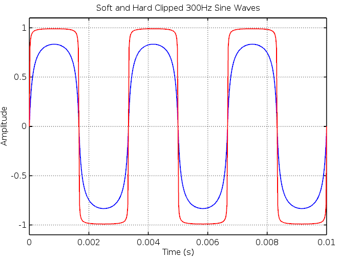
First, lets introduce our sine sweep as the signal $x$ and recorded measurement as $y$ . We can then write their respective Fourier transforms as:

(1) $\begin{gather*} X=\mathcal{F}\{x\} \\ Y=\mathcal{F}\{y\}.\end{gather*}$

The deconvolution provides a numerical frequency response (or transfer function), $H$ , and is calculated as the division of the measured frequency spectrum, $Y$ by the input frequency spectrum, $X$ :

(2) $\begin{equation*}H = \frac{Y}{X}.\end{equation*}$

The big advantage of deconvolution is that the input signal doesn’t have to be a sine sweep; acceptable results can, in theory, be found just by recording the input/output response of a short jam session, white noise, or a series of impulse functions. Each test signal has its own advantages and all are used in different acoustic measurements contexts.

Modelling Via Time Domain Least Squares Regression

Plots in this section can be recreated by running the GNU Octave code in this archive. The archive also contains the measured sine sweep .wav file.

We attempted to create a high order IIR filter using a linear least squares regression method assuming that a general 8th order system (8 zeros, 8 poles) had generated the output $y$ from the input $x$ . This procedure takes the measured time domain data from the .wav files and, via a substantial amount of linear algebra, calculates IIR filter coefficients which best fit the given time domain input/output data.

The frequency response of the model this method created is shown below on a linear frequency scale:

—-
Update 31st Jan 2019: A major omission here was to neglect any pure time delay introduced by the speaker – mic air gap. A 10cm gap sampling at 48 kHz is about 14 samples delay. This introduces significant modelling error when building IIR filters.
—-

It can be seen that the models match reasonably well however there is substantial error below 1kHz. This modelling error is easily seen when viewing the above data with a logarithmic frequency axis:

This model (red) misses the speaker’s bass peak at ~130Hz and leaves a big gap in the upper mid range ~800-1000Hz. Furthermore, there is a significant amount of detail (poles and zeros) around 10kHz which, for the purposes of a guitar signal, is wasted as there is typically a low amount of energy present in that frequency range.

We strongly suspect that the poor low frequency fit is due to numerical precision limits in the least squares calculation. This problem stems from IIR filters suffering from numerical noise at low frequency, an issue which is exacerbated by increasing filter’s order. As such, the 8th order system cannot be accurately evaluated at low frequency, resulting in the poor model fit.

This problem is solved in the Vector Drive pedal by passing the signal through four 2nd order filters instead of a single 8th order one. Unfortunately this method does not help when building the system model.

The regression model does, however, provide an excellent starting point from which manual (or automated) adjustments can be made. Future work may involve, say, a time domain least squares analysis followed by a frequency domain stochastic optimiser such as simulated annealing.

The manual tweaking method used below takes account of the fact that the speaker’s low to midrange response makes a substantial difference to the amp’s tone. By manually curve fitting these tonal features we build a much more faithful reproduction of the speaker’s timbre.

Hand Tuning the Model

Given the cabinet’s measured frequency response and rough starting point for the filters we optimised the system by hand. We kept the 8th order system (four 2nd order sections in series) and constrained them with the following broad features:

A 2nd order high pass filter (2 poles around 130Hz, 2 zeros at the origin)
Two arbitrary peaking/shelving filters (2 poles and 2 zeros in the 500-2000Hz range)
A 2nd order low pass filter (2 poles around 5000Hz).

Using an Octave script for visualisation the filters were manually tuned until the filter’s response roughly followed the data points. The final result is superimposed over the speaker’s frequency response in the graph below:

Final Filter Coefficients

We’re happy for you to have a play with the filter we built. The final coefficients can be loaded into Octave or MATLAB with the following code:

% Vector Drive cabinet emulation filters
% Copyright Z Squared DSP Pty Limited
% Permission is granted for non-commercial use of these filters

b1 = [0.998427797774257 -1.996855595548515 0.998427797774258];
a1 = [1.000000000000000 -1.996729031901556 0.996982159195472];

b2 = [1.71381752013609 -3.59123502602204 1.89042101128582];
a2 = [1.000000000000000 -1.946518614625237 0.959522120025104];

b3 = [2.44712046192491 -5.07920063666641 2.71162250478877];
a3 = [1.000000000000000 -1.847874331025749 0.92741666107301];

b4 = [0.0744394809810769 0.1488789619621539 0.0744394809810770];
a4 = [1.000000000000000 -1.433046457023383 0.730804380947690];

In Octave a digital IIR filter is defined by two row vectors (arrays): b and a. Those two vectors can be passed as arguments to the filter() function. So, if you have a recording in a 48kHz .wav file called ‘input.wav’ you can run it through our cab emulation by running the variable declarations above followed by this code:

% input.wav MUST be sampled at 48kHz!
Fs = wavread('input.wav');

y1 = filter(b1, a1, x);
y2 = filter(b2, a2, y1);
y3 = filter(b3, a3, y2);
y4 = filter(b4, a4, y3);

wavwrite(y4, 48e3, 'output.wav');

The output will be written to ‘output.wav’.

If using MATLAB wavread() and wavwrite() need to be substituted with the audioread() and audiowrite() functions.