This post covers the creation of infinite impulse response filters which emulate guitar speaker cabinets. A follow-up post covers the creation of more accurate, but far more computationally intensive, impulse response models.
Introduction
On the Vector Drive’s long list of features is cabinet emulation; the ability of the pedal to generate an output which sounds like it is coming from a real amp’s speaker cabinet. This is done by passing the output audio through a series of filters which mimic the tonal properties of a guitar speaker we have in the Z Squared DSP studio: a Blackheart BH112 1×12″ driven by a Little Giant 5 tube head.
This post describes the method we used to tune the cabinet emulation system, a series of four second order infinite impulse response (IIR) filters. These are digital signal processing (DSP) filters which models analog RLC circuits and are used here because of their computational efficiency and low latency. If you’ve used digital audio workstation cab emulation plugins they may instead use finite impulse response (FIR) filters or even convolutions. These methods can be more accurate but typically introduce unacceptably high delays (ie: they aren’t real-time methods) and are far too computationally intensive for the humble DSP microcontroller in the Vector Drive.
The goal of our cabinet modelling procedure was therefore to create a high order IIR filter which closely approximated the sinusoidal steady state response of the BH112 speaker cabinet. This model ignores any non-linear (distortion) effects of the speaker/amp combo (ie: measurements are performed at a low-ish volume) and only applies to a single microphone location.
Audio Samples
Before diving into the details have some audio samples, this is probably what most readers are here for anyway. The following clips compare the same audio with & without cabinet emulation applied.
Clean Riff Raw
Clean Riff Emulated
Distorted Riff Raw
Distortion Riff Emulated
Method Overview
The basic steps required to build a speaker cabinet model are:
- Measure the frequency response of the speaker
- Create a filter which matches this response by eye
- Perform listening tests and tweak the filter as necessary.
Cabinet Measurements
The speaker’s frequency response was measured by injecting a logarithmically varying sinusoidal sweep (chirp signal) into the amp while simultaneously recording the speaker’s output. We used a 60 second long 20Hz to 20kHz sine sweep generated by Audacity and a Marantz MPM1000 condenser microphone. The studio’s RT60 is about 250ms and the sweep is slow enough that influence from the room’s dynamics are minimised.
A more accurate model would be found by using a calibrated microphone inside an anechoic chamber but in the end we’re not trying to copy the BH112, just use it as a guide when creating a model that sounds better than the raw output for driving headphones or doing DI injection at a live gig. Everyone has their own speaker preference and we aren’t trying to create a catalog of speaker cab models…yet ;).
Prior to recording the sine sweep the microphone’s placement was optimised using subjective listening tests during a jam session. Mic placement has a huge influence on the tone but we aren’t trying to model that effect here.
At the end of the generated sine sweep track we included a few metronome ticks so that the sweep track could be accurately be aligned with the recording. This is crucial for model accuracy when attempting the time domain least squares regression method in the next section as it assumes that the amp’s input and speaker output are measured simultaneously. After temporal alignment the metronome clicks were removed and the two tracks exported as .wav files.
The generated chirp and recorded speaker response can be found in this archive in the file sine_measurement.wav.
Frequency Analysis
The speaker’s frequency response is calculated with a method known as a deconvolution. This method takes into account the unequal energies in the input frequency spectrum which result from using a log frequency swept sinusoidal test signal.
First, lets introduce our sine sweep as the signal  and recorded measurement as
  . We can then write their respective Fourier transforms as:
(1) 
The deconvolution provides a numerical frequency response (or transfer function),  , and is calculated as the division of the measured frequency spectrum,
  by the input frequency spectrum,
  :
:
(2) 
The big advantage of deconvolution is that the input signal doesn’t have to be a sine sweep; acceptable results can, in theory, be found just by recording the input/output response of a short jam session, white noise, or a series of impulse functions. Each test signal has its own advantages and all are used in different acoustic measurements contexts.
Modelling Via Time Domain Least Squares Regression
Plots in this section can be recreated by running the GNU Octave code in this archive. The archive also contains the measured sine sweep .wav file.
We attempted to create a high order IIR filter using a linear least squares regression method assuming that a general 8th order system (8 zeros, 8 poles) had generated the output from the input . This procedure takes the measured time domain data from the .wav files and, via a substantial amount of linear algebra, calculates IIR filter coefficients which best fit the given time domain input/output data.
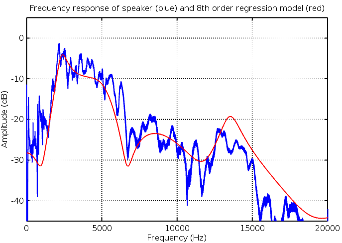
The frequency response of the model this method created is shown below on a linear frequency scale:
—-
Update 31st Jan 2019: A major omission here was to neglect any pure time delay introduced by the speaker – mic air gap. A 10cm gap sampling at 48 kHz is about 14 samples delay. This introduces significant modelling error when building IIR filters.
—-
It can be seen that the models match reasonably well however there is substantial error below 1kHz. This modelling error is easily seen when viewing the above data with a logarithmic frequency axis:
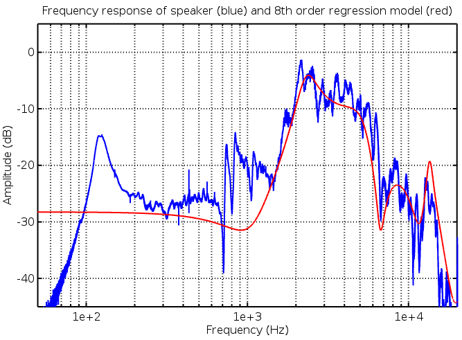
This model (red) misses the speaker’s bass peak at ~130Hz and leaves a big gap in the upper mid range ~800-1000Hz. Furthermore, there is a significant amount of detail (poles and zeros) around 10kHz which, for the purposes of a guitar signal, is wasted as there is typically a low amount of energy present in that frequency range.
We strongly suspect that the poor low frequency fit is due to numerical precision limits in the least squares calculation. This problem stems from IIR filters suffering from numerical noise at low frequency, an issue which is exacerbated by increasing filter’s order. As such, the 8th order system cannot be accurately evaluated at low frequency, resulting in the poor model fit.
This problem is solved in the Vector Drive pedal by passing the signal through four 2nd order filters instead of a single 8th order one. Unfortunately this method does not help when building the system model.
The regression model does, however, provide an excellent starting point from which manual (or automated) adjustments can be made. Future work may involve, say, a time domain least squares analysis followed by a frequency domain stochastic optimiser such as simulated annealing.
The manual tweaking method used below takes account of the fact that the speaker’s low to midrange response makes a substantial difference to the amp’s tone. By manually curve fitting these tonal features we build a much more faithful reproduction of the speaker’s timbre.
Hand Tuning the Model
Given the cabinet’s measured frequency response and rough starting point for the filters we optimised the system by hand. We kept the 8th order system (four 2nd order sections in series) and constrained them with the following broad features:
- A 2nd order high pass filter (2 poles around 130Hz, 2 zeros at the origin)
- Two arbitrary peaking/shelving filters (2 poles and 2 zeros in the 500-2000Hz range)
- A 2nd order low pass filter (2 poles around 5000Hz).
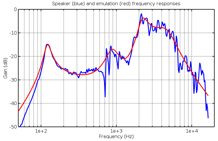
Using an Octave script for visualisation the filters were manually tuned until the filter’s response roughly followed the data points. The final result is superimposed over the speaker’s frequency response in the graph below:

Final Filter Coefficients
We’re happy for you to have a play with the filter we built. The final coefficients can be loaded into Octave or MATLAB with the following code:
% Vector Drive cabinet emulation filters
% Copyright Z Squared DSP Pty Limited
% Permission is granted for non-commercial use of these filters

b1 = [0.998427797774257 -1.996855595548515 0.998427797774258];
a1 = [1.000000000000000 -1.996729031901556 0.996982159195472];

b2 = [1.71381752013609 -3.59123502602204 1.89042101128582];
a2 = [1.000000000000000 -1.946518614625237 0.959522120025104];

b3 = [2.44712046192491 -5.07920063666641 2.71162250478877];
a3 = [1.000000000000000 -1.847874331025749 0.92741666107301];

b4 = [0.0744394809810769 0.1488789619621539 0.0744394809810770];
a4 = [1.000000000000000 -1.433046457023383 0.730804380947690];
In Octave a digital IIR filter is defined by two row vectors (arrays): b and a. Those two vectors can be passed as arguments to the filter() function. So, if you have a recording in a 48kHz .wav file called ‘input.wav’ you can run it through our cab emulation by running the variable declarations above followed by this code:
% input.wav MUST be sampled at 48kHz!
Fs = wavread('input.wav');

y1 = filter(b1, a1, x);
y2 = filter(b2, a2, y1);
y3 = filter(b3, a3, y2);
y4 = filter(b4, a4, y3);

wavwrite(y4, 48e3, 'output.wav');
The output will be written to ‘output.wav’.
If using MATLAB wavread() and wavwrite() need to be substituted with the audioread() and audiowrite() functions.